This portion of the web site contains formulas and procedures for the descriptive statistics noted below.
A useful and simple way to summarize group data that is categorical or ordinal scaled is to construct a frequency distribution table.
To make a frequency distribution table (fdt) simply list each raw score (x) observed followed by a count (also called absolute frequency) of the number of individuals with that score. An additional column called the relative frequency is often useful since it notes the percentage of the group with a particular raw score.
Ex: 6,4,6,2,8,3,3,6
x f rf 8 1 12.5% 6 3 37.5% 4 1 12.5% 3 2 25% 2 1 12.5% x: raw score
f: absolute frequency - count
rf: relative frequency - count/N (100) - record as %
If a frequency distribution table is needed when the data set is very large, comprised of at least interval scaled data, and scores very spread out, it is often necessary to create an intervaled frequency distribution table. Rules guide the construction of the 1st interval then all other intervals can be listed in numerical order following the 1st interval. Across from the interval you would record the number of individuals with scores in that interval.
To construct the 1st interval:
(a) calculate an interval size (IS).

HS = High Score; LS = Low Score
(b) Design the 1st interval so it contains the highest score somewhere in the interval and:
- if IS is even, the smallest score in the
interval should be divisible by the IS.
For Example: if HS=98 and LS=38 then:
so, the 1st interval would be 96-99 since 96 is the only number divisible by 4 that can be listed first in the interval and still contain the high score (98). The rest of the Ifdt would be constructed by listing intervals (of size 4) below the first one until the low score is contained in the last interval.
x f 96-99 92-95 88-91 84-87 80-83 76-79 72-75 68-71 64-67 60-63 56-59 52-54 48-51 44-47 40-43 36-39
- if IS is odd, the middle score in the interval should be divisible by the IS.
For Example: if HS=86 and LS=12 then

so, the 1st interval would be 83-87 since 85 is the only number divisible by 5 that can be listed in the middle and still have the interval contain the high score (86). The rest of the Ifdt would be constructed by listing intervals (of size 5) below the first one until the low score is contained in the last interval.
Central Tendency: A measure of central tendency locates the middle or center of a distribution.
Note: when information is drawn from an intervaled fdt it can be misleading. Measures of central tendency should be determined directly from the raw data. Not from an intervaled frequency distribution table.
Measures:
Mode - Score that occurs most frequently
Median - Score that separates group into equal halves (middle score)
Mean - Arithmetic average of a set of scores
You decide which to use based on: Level of Measurement, Shape of distribution, Need for accuracy.
What to use when:
Determining the Mode: Select score (x) from
a frequency distribution table with highest frequency.
| x | f | |
| 12 | 1 | |
| 10 | 3 | |
| 9 | 5 | |
| 7 | 1 |
The score with the highest frequency is 9, so the Mode in this data set is 9.
Determining the Median:
1. Locate general position of middle score on a frequency distribution table. .50(N) scores must be below and above the middle score.
2. Draw a line on the frequency distribution table that locates the midpoint.
If frequency at the line = 0, then interpolate (meaning select the midpoint between the two numbers you drew the line between).
x f 12 1 10 1 9 1 7 1 Median = 9.5
If frequency at the line = 1, the x value at the line is the median
x f 12 1 10 1 9 1 7 1 6 1 4 1 2 1 Median = 7
If frequency at the line > 1 you have a decision to make: If you want an approximate median, the x value at the line is the median. If you want an exact median, you use a formula.

LrL = lower real limit = x at line - .50
N = total number of scores/people
fb = number of scores below line
fw = frequency at line
Example:
x f 6 1 5 2 4 3 3 2 2 2 Mdn = 3.5 +(5-4/3) = 3.83
Note: Remember to list scores from best to poorest. It is also
helpful (not necessary) to add a cumulative frequency column.
Example:
| x | f | cf | ||
| 6 | 1 | 10 | ||
| 5 | 2 | 9 | ||
| 4 | 3 | 7 | ||
| 3 | 2 | 4 | ||
| 2 | 2 | 2 |
f at line for this data set is > 1 so, need to use the formula
to compute an exact median. The approximate median is the x value (4) you draw
your line through. The exact median is:

Another Example:
| x | f | cf | ||
| 18 | 1 | 12 | ||
| 14 | 2 | 11 | ||
| 12 | 5 | 9 | ||
| 10 | 2 | 4 | ||
| 8 | 2 | 2 |
Since the frequency at the line (line through 12) is > 1, you need formula to compute an exact median:
Another Example:
| x | f | cf | ||
| 80 | 8 | 31 | ||
| 75 | 4 | 23 | ||
| 72 | 12 | 19 | ||
| 70 | 7 | 7 |
Since the frequency at the line (line through 72) is > 1, you need to use the formula to compute an exact median:
| x | f | cf | ||
| 12 | 2 | 40 | ||
| 11 | 8 | 38 | ||
| 6 | 10 | 30 | ||
| 4 | 8 | 20 | ||
| 2 | 7 | 12 | ||
| 1 | 5 | 5 |
In this case, you draw the line between the 4 and 6 and since the frequency at the line is zero you interpolate: Mdn = 5
Another Example:
| x | f | cf | ||
| 80 | 3 | 25 | ||
| 74 | 2 | 22 | ||
| 72 | 7 | 20 | ||
| 70 | 5 | 13 | ||
| 65 | 4 | 8 | ||
| 63 | 4 | 4 |
Since the frequency at the line (line through 70) is > 1, you need to use the formula to compute an exact median:

Another Example:
| x | f | cf | ||
| 85 | 3 | 13 | ||
| 80 | 1 | 10 | ||
| 72 | 2 | 9 | ||
| 70 | 1 | 7 | ||
| 68 | 3 | 6 | ||
| 61 | 3 | 3 |
Since the frequency at the line = 1 (line through 70), Median = 70
Determining the Mean: To calculate the mean

| x | f | |
| 8 | 2 | |
| 4 | 1 | |
| 3 | 3 | |
| 1 | 4 |
Note: You must remember to take the frequency into consideration - there are two scores of 8, one score of 4, three scores of 3, and 4 scores of 1. The sum of these raw scores is 33 and there are a total of ten scores so the mean is:

Another Example:
| x | f | |
| 14 | 1 | |
| 7 | 3 | |
| 5 | 3 | |
| 3 | 2 | |
| 2 | 1 |

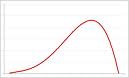
Relationships among measures of central tendency:

Measures of variability reflect how scores vary (how spread
out) around the center of a distribution.
Spread of scores from high to low. Not very stable since it uses only 2 scores and is affected by changes in either. Also is not sensitive to the center or shape of the distribution.
Signed Deviation: The signed (+) distance a raw score is from the mean. Useful for describing position in a group but, can't be averaged to get an overall average group deviation since signed deviations always sum to zero.
![]()
| x | f | d | ||
| 18 | 1 | 18-10=8 | ||
| 12 | 1 | 12-10=2 | ||
| 7 | 1 | 7-10= -3 | ||
| 3 | 1 | 3-10= -7 |
Standard deviation: Average unsigned distance of a set of raw scores from their mean. Most commonly reported measure of variability for continuous variables.
A large value for Sx means that scores on the average
are a greater distance from their mean. Sx also has the characteristic
that the entire range of scores lies between mean + 3(Sx).
Ex: when mean = 4.25 and Sx = .97, you know no one scored higher
than 4.25 + 2.91 and no one scored lower than 4.25 - 2.91.
Definitional formula:

Xi = score for an individual
N = number of individuals in group
Computational formula:
Example:
| x | f | |
| 18 | 1 | |
| 12 | 1 | |
| 7 | 1 | |
| 3 | 1 |

Another Example:
| x | f | |
| 6 | 2 | |
| 5 | 3 | |
| 4 | 9 | |
| 3 | 1 | |
| 2 | 1 |
Mean = 68/16 = 4.25

Examples of all measures of central tendency & variability:
| x | f | |
| 10 | 5 | |
| 8 | 2 | |
| 6 | 1 | |
| 4 | 1 | |
| 1 | 2 |
Mode = 10
Mean = 78/11 = 7.09

![]()
![]()

Percentile Ranks: Provide information on what % of a group scored below a given raw score.
Steps in calculating Percentile Ranks:
![]()
Example:
| x | f | cf | PR | |||
| 10 | 1 | 25 | 98% | |||
| 6 | 4 | 24 | 88% | |||
| 5 | 10 | 20 | 60% | |||
| 4 | 6 | 10 | 28% | |||
| 3 | 3 | 4 | 10% | |||
| 0 | 1 | 1 | 2% |
Calculations for the Percentile Ranks of the raw scores of 6 and 10 follow:
![]()
![]()
Another Example:
| x | f | cf | PR | |||
| 82 | 7 | 24 | 85% | |||
| 75 | 4 | 17 | 63% | |||
| 70 | 1 | 13 | 52% | |||
| 64 | 3 | 12 | 44% | |||
| 60 | 8 | 9 | 21% | |||
| 58 | 1 | 1 | 2% |
To determine the Percentile Rank of the raw score 60:
![]()
Percentiles: Provides the raw score associated with a given percentile rank. Tells you what raw score has a specified percentage of the group below it.
Note: Consider the median . . . It is the score that divides the group in half. You could say this is the raw score associated with a percentile rank of 50% (or the 50th percentile - 50P). Therefore, the formula used to determine the median should be useful in determining any percentile.
Steps:

Example:
| x | f | cf | ||
| 12 | 8 | 20 | ||
| 7 | 6 | 12 | ||
| 6 | 1 | 6 | ||
| 4 | 3 | 5 | ||
| 3 | 2 | 2 |
To determine the 40th Percentile: .40(20) = 8, so
draw line through 7. Since the frequency at the line is >1, use formula:

To determine the 20th Percentile: .20(20) = 4, so
draw line through 4. Since the frequency at the line is >1, use formula:

Another Example:
| x | f | cf | ||
| 77 | 2 | 22 | ||
| 64 | 3 | 20 | ||
| 60 | 5 | 17 | ||
| 51 | 4 | 12 | ||
| 50 | 3 | 8 | ||
| 47 | 2 | 5 | ||
| 18 | 3 | 3 |
Mean = 52.18 Sx = 15.86
To determine the Percentile Rank of the raw score 60:

To determine the Percentile Rank of the raw score 47:
![]()
To determine the 70th Percentile: .70(22) = 15.4,
so draw line through 60, then:

Transformations: x to z; z to x
A standardized score is a transformed score no longer written in terms of the original raw score units. After the transformation, a standard score gives information regarding the position of the original raw score relative to the mean.
Standard scores are essential for combining scores coming from
different scales or scores with different units of measurement. Standard scores
are also a shorthand way of communicating information about performance relative
to a reference group. The two most common types of standard scores are z scores
and t scores. The transformation of scores from one scale to another is accomplished
using what can be referred to as a generic transformation formula:
![]()
Note: While the generic transformation formula provides an excellent
cookbook approach to transformations, the concept should not be overlooked.
In all transformations the transformed score must precisely reflect the actual
distance and direction from the original mean.
z scores have a mean of 0 and standard deviation
of 1 [always]. To transform a raw score to a z score the generic formula can
be used:

Since Sz = 1 and the mean = 0, the formula can be simplified to:

Example: raw score mean = 20 and Sx = 5. Transform x = 15 to a z score.

Anther example: Given a group with a Mean = 60 and Standard deviation = 12;
if x = 80, z = ?

The z score itself with no other information conveys the distance and direction of a raw score from its mean. Therefore z scores are a convenient way to provide relative information regarding a person's position with respect to some reference group. Two of the most common applications, given this characteristic of z scores is for the data profiling of performance and for transforming scores before a grade is assigned (curving scores).
To reverse the process and transform a z to a raw score, the
generic formula becomes::

Since the mean and standard deviation for z scores are 0 and
1, the generic formula is simplified to:
Example: Given a raw score mean of 45 and standard deviation of 3,
if z = 2.8, x = ?
![]()
if z = -.50, x = ?
![]()
Another Example: Given a group Mean = 14 and Standard deviation = 2.3,
if z = 1.80, x = ?
x = 2.3(1.80) + 14 = 18.14
if z = -2.4, x = ?
x = 2.3(-2.4) + 14 = 8.48
Correlational analyses allow you to examine the strength of the relationship between two variables. Correlation coefficients help you answer questions like 'Do students with high IQ scores achieve better college grades?' The underlying question can be phrased: is there a relationship between IQ and GPA.
There are several types of correlation coefficients to choose from. The choice is based on the nature of the variables being correlated.
| Pearson Product Moment Correlation | Use when both variables continuous | ||
| Phi | Use when both variables dichotomous | ||
| Point Biserial | Use when one continuous and one dichotomous | ||
| Kendall's Tau | Use when both variables ordinal (ranks) |
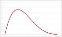
A Pearson Product Moment Correlation (PPMC) coefficient describes the strength and direction of the linear relationship between two variables. When two variables are not linearly related, the PPMC is likely to underestimate the true strength of the relationship. A graph of the x and y values should be examined to determine whether or not the relationship is linear.
When the scores on two variables get larger/smaller together, the direction of the relationship is positive. When scores on one get larger as scores on the other variable get smaller, the direction of the relationship is negative due to the inverse relationship of the two variables. When there is no pattern, there is no relationship and the correlation coefficient is zero.
A PPMC coefficient is a signed number between -1 and 1 where 0 represents no relationship. Presence of a relationship should never be interpreted as demonstrating cause and effect. Remember the negative sign simply conveys direction. The farther away from zero in either direction the stronger the relationship.
The PPMC is affected by the variability of the scores collected. Other things being equal, the more homogeneous the group (on the variables being measured) the lower the correlation coefficient. Since small groups tend to be more homogeneous, Pearson is most meaningful and most stable when group size is large (>50).
The computational formula for the PPMC is

Example:
| x | y | |
| 5 | 10 | |
| 4 | 9 | |
| 3 | 8 | |
| 2 | 7 | |
| 1 | 6 |

A point biserial correlation coefficient tells you the strength of the relationship between one continuous and one dichotomous variable. The sign carries little meaning. It only indicates which group tended to have higher scores. The point biserial coefficient is a signed number between -1 and 1 where again zero represents no relationship.
The computational formula for the point biserial coefficient is

Where:
X0 = mean of x values for those in category 0
X1 = mean of the x values for those in category 1
Sx = standard deviation of all x values
P0 = proportion of people in category 0
P1 = proportion of people in category 1
To obtain the components you need from SPSS so you can do Point Biserial by hand, you would:
Example: Is there a relationship between height, defined as short and tall, and quiz scores? Assume those in category 1 are < 5'5" and those in category 0 are > 5'5"
| Quiz Score | Group | |
| 6 | 0 | |
| 8 | 0 | |
| 4 | 1 | |
| 2 | 1 | |
| 1 | 0 |

point biserial correlation = -.38
A phi correlation coefficient tells you the strength of the relationship between two dichotomous variables. The sign carries little meaning. It only indicates which diagonal had the greater concentration of scores. The phi coefficient is a signed number between -1 and 1 where again zero represents no relationship.
To estimate phi,
(a) set up a two by two table
y a b x c d
(b) use the computational formula for phi:

Example: What is the strength of the relationship between gender and athletic participation? (gender: 0=male, 1=female; athletics: 0=no, 1=yes)
| Gender | Athletics | |
| 0 | 1 | |
| 1 | 1 | |
| 1 | 1 | |
| 0 | 0 | |
| 1 | 0 | |
| 1 | 0 | |
| 1 | 0 | |
| 1 | 1 | |
| 0 | 0 | |
| 0 | 1 | |
| 1 | 0 | |
| 0 | 1 | |
| 0 | 1 | |
| 1 | 0 | |
| 0 | 1 |
set up a two by two table
athletic participation No Yes Male 2 5 gender Female 5 3
Calculate phi:

The phi correlation reflects a low negative (inverse) relationship between gender and athletic participation. The pattern this correlation coefficient detected is that there is some tendency for men to be more likely to participate in athletics and women not to participate.
Since the correlation coefficient measures the strength of the relationship between two variables it can be used along with other descriptive statistics to predict the value of one variable from another. This discussion will be limited to predicting one continuous variable from another continuous variable. Therefore, the PPMC will be the correlation coefficient employed.
Steps:

For example: Given this information:
| Mean | Standard Deviation | ||||
| x | 20 | 5 | |||
| y | 35 | 10 |
Assume PPMC = .80
If x = 30, what do you predict y will be?

Prediction is accurate only when the individual is similar to the group the correlation came from with respect to age, gender, ability and any other important characteristic. To be considered similar with respect to ability, the individual's score must be within 3 standard deviations of the mean. From example, x had to be between 5 and 35 in the example above.
Note: The weaker the correlation, the more error there is in predicting a y score. The amount of error to be expected can be quantified using a statistic called the Standard error of estimate:
![]()
For example, if the standard deviation for the variable being predicted (y) is 10 and the correlation between x and y = .80, then the standard error of estimate is:
![]()
You interpret SEE relative to the standard deviation of the y scores. If SEE close to Sy there's a lot of error in prediction.
Individual & Group Profiles
To profile performance measures for a group or individual
In the case of an individual compared to a relative standard (eg. state mean):

In the case of a group (eg. district mean) compared to a relative standard (eg. state mean):
To profile indiviual/group measures compared to both relative and criterion-referenced standards:
In the case of an individual compared to a relative standard (eg. state mean):
In the case of a group (eg. district mean) compared to a relative standard (eg. state mean):
For example: Assume you have collected sit-up and 50 yard dash times. The individual you want to construct a profile for did 24 sit-ups (in 30 seconds) and had a dash time of 7 seconds. Also, assume the reference group (eg. the class the student was tested with) measures and criterion measures were:
Class Mean Class Standard Deviation Criterion Sit-up 17 4 20 50 yard Dash 7.8 .30 8
Transforming the individual's sit-up score to a z score:
Transforming the individual's dash score to a z score:
Note, since low dash scores reflect good performance, for the purpose of visual feedback you would switch the sign on the dash information before putting it on a graph.
Transforming the criterion sit-up score to a z score:
Transforming the criterion dash score to a z score:
Note, since low dash scores reflect good performance, for the purpose of visual feedback you would switch the sign on the dash information before putting it on a graph.
From a profile constructed this way you will have a visual representation of how (a) individual performance compared to the group, (b) individual performance compared to the criterion, and (c) group performance compared to the criterion. In this example:
- The individual performed better than the group on both measures
- The individual exceeded the criterion on both measures
- The group exceeded the dash criterion and scored below the sit-up criterion
Note: Profiling is an appropriate technique for communicating performance in any domain.
Two statistics are calculated in a classical item analysis:
Difficulty Index: A measure of how difficult the item was for the group tested.

As the intention for an item changes to be more or less difficult the acceptable and optimal values change according to the intention of the item writer. There are general guidelines to consider.
Test Score Item Score 82 1 70 0 91 1 80 1 74 0 80 1 93 1 60 0 68 0 78 1

Discrimination Index: A measure of the effectiveness of an item in discriminating among ability levels in the group tested.
Two procedures for calculating discrimination indices:

x1 = Mean test score
of individuals getting item correct
x2 = Mean test score of individuals missing item
p1 = Proportion of group getting item correct
p2 = Proportion of group missing item
Test Score Item Score 82 1 70 0 91 1 80 1 74 0 80 1 93 1 60 0 68 0 78 1

Assuming this was intended to be a moderately difficult item based on the discrimination index (.82) and difficulty index (.60) this was a good item.
Difference in proportions: Use the top and bottom 27% of the group (based on overall test score) and compare them. If the item worked well the majority of the top group will get the item correct and the majority of the bottom group will miss the item.
![]()
Optimal value for correct choice > .40
Acceptable value for correct choice > .30
Optimal value for distractor < -.20
Acceptable value for distractor < 0
A B* C D 0 4 0 1 Top 27% 1 1 2 1 Bottom 27%
Dp(D) = 1/5 - 1/5 = 0
Based on only the discrimination indices, this is a good item.
A B C* D 1 2 7 2 Top 27% 3 4 2 3 Bottom 27%
Dp(D) = 2/12 - 3/12 = -.08
The final interpretation of an item's effectiveness depends on what you intended. Very hard items are needed to discriminate at the A/B level and easy items are needed to discriminate at the D/F level.
To be complete the item analysis should include difficulty for the item overall and discrimination indices on the correct choice and distractors. Close examination of item indices is essential in order to revise weak items before using them again. An item analysis is very useful for identifying what needs to be done to improve a test and subsequently improve reliability of the scores.
The Differences in proportion results should be interpreted with care since the N the answers are based on can be fairly small and you have lost all the information from the middle third of the group
For traditional tests, other things being equal, the higher the average discrimination index (across all items) the better the reliability; and the closer the average difficulty index to .50 the better the reliability.
Mastery tests are designed to place examinees into one of two categories master/non-master based on a cut score. An item analysis for a mastery test examines the same two indices - difficulty and discrimination. However, with discrimination, different statistics are required because you are no longer interested in distinguishing among ability levels only distinguishing between two groups - master/non-master.
Difficulty Index: A measure of how difficult the item was for the group tested.
Range for difficulty indices: 0 to 1
Since you still need a range of items from easy to difficult in order to accurately classify individuals as masters or nonmasters the same rules can be applied:
The one point to keep in mind overall for mastery tests is that in general the closer the average difficulty index to the groups' ability the more likely reliability will be diminished.
Discrimination index: A measure of how well an item distinguishes between masters and non masters
Two choices:
Item Score correct incorrect master a b Test Classification non-master c d
Item Score correct incorrect master A B Test Classification non-master C D

Test Score Classification Item Score 20 Master 1 15 Master 0 16 Master 1 16 Master 1 12 Non-master 0 11 Non-master 0 14 Non-master 0 12 Non-master 1
Item Score correct incorrect master 3 1 Test Classification non-master 1 3
D = 4/8 = .50


Based on these item indices, this was a good item.